
math
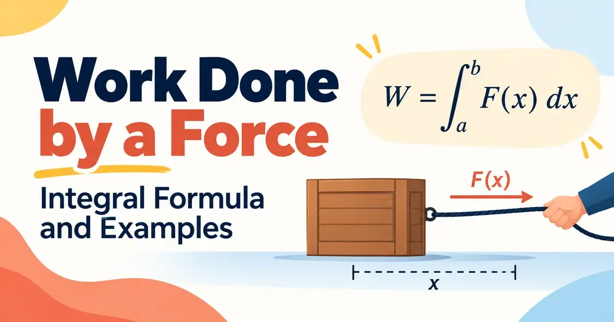
Work Done by a Force: Integral Formula and Examples
Calculus
math
Surface Area of Revolution: Formula and Examples
Calculus
math
Volumes by Slicing: Cross Sections and Examples
Calculus
math
Sum and Difference Rule for Derivatives and Integrals
Calculus
math
Quadratic Approximation: Formula, Error, Examples
Calculus
math
One-Sided Limits: Left-Hand and Right-Hand Limits
Calculus
math
Notation for Differentiation: Leibniz, Lagrange, Newton
Calculus
math
Modeling with Differential Equations: Steps and Examples
Calculus
math
List of Integrals of Trigonometric Functions: Full Table
Calculus
math
List of Integrals of Logarithmic Functions With Proofs
Calculus
math
List of Integrals of Rational Functions With Proofs
Calculus
math
List of Integrals of Inverse Trigonometric Functions
Calculus
math
List of Integrals of Irrational Functions With Examples
Calculus
math
List of Integrals of Hyperbolic Functions: Full Tables
Calculus
math
Linear Approximation and Local Linearization Explained
Calculus
math
List of Integrals of Exponential Functions With Proofs
Calculus
math
L'Hôpital's Rule: Conditions, Forms and Examples
Calculus

math
Limits of Piecewise Functions: Steps and Examples
Calculus
math
Leibniz Newton Calculus Controversy: Timeline and Verdict
Calculus
math
Inverse Chain Rule Method: Reverse Chain Rule Integration
Calculus
math
Introduction To Limits: Meaning, Notation, Examples
Calculus
math
Introduction to Integration: Meaning, Rules, Examples
Calculus
math
Introduction to Differential Equations: Types, Examples
Calculus
math
Introduction to Derivatives: Meaning, Rules, Examples
Calculus
math
Integration Using Reduction Formulas: Steps, Examples
Calculus
math
Integration of Logarithmic Functions With Examples
Calculus
math
Integration of Irrational Functions: Methods & Examples
Calculus
math
Infinitesimal Calculus: Meaning, History and Examples
Calculus
math
Infinite Limits: Definition, Asymptotes and Examples
Calculus
math
Higher-Order Derivatives: Notation, Patterns, Examples
Calculus
math
General Leibniz Rule: Formula, Proof and Examples
Calculus
math
Graphs And Limits: Reading Limits From A Graph
Calculus
math
General and Particular Solutions: Definitions, Examples
Calculus
math
First-Order Differential Equations: Types and Methods
Calculus
math
Evaluating Limits Algebraically: Methods and Examples
Calculus
math
Differential of a Function: Formula, Examples, Errors
Calculus
math
Euler's Number (e): Definition, Value and Proofs
Calculus
math
Derivatives of Hyperbolic Functions: Formulas & Proofs
Calculus
math
Derivatives of a Function in Parametric Form Explained
Calculus
math
Derivative as Slope of a Tangent Line: Formula, Examples
Calculus
math
Convex and Concave Functions: Definition and Tests
Calculus
math
Convergent and Divergent Sequences: Tests and Examples
Calculus
math
Convergence Tests: Which Series Test to Use and When
Calculus
math
Continuity on an Interval: Endpoint Rules and Examples
Calculus
math
Constant Rule: Why The Derivative Of A Constant Is 0
Calculus
math
Calculus with Python: SymPy and NumPy Guide
Calculus
math
Concavity and Points of Inflection: Steps and Examples
Calculus
math
Calculus Symbols and Notation: List, Meaning
Calculus
math
Branches of Calculus: Types, Uses and Examples
Calculus
math
Bounded Sequences: Definition, Sup, Inf and Examples
Calculus
math
Average vs Instantaneous Rate of Change Explained
Calculus
math
Archimedes and Early Infinitesimals: The Road to Calculus
Calculus
math
Applications of Calculus in Real Life, With Examples
Calculus
math
Center of Mass and Centroid: Formulas and Examples
Calculus
math
Volume Of Solids Of Revolution: Disk, Washer, Shell
Calculus
math
Washer Method: Volume Of Revolution Formula
Calculus
math
Velocity and Acceleration: Calculus Derivatives
Calculus
math
History of Calculus: Timeline From Archimedes to Newton
Calculus
math
Types Of Discontinuity: Removable, Jump & Infinite
Calculus
math
Taylors Theorem: Formula, Remainder & Examples
Calculus
math
Transformations Of Functions: Rules & Examples
Calculus
math
Tangent Line Equations: Formula, Steps & Examples
Calculus
math
Table of Integrals: Standard Formulas & Examples
Calculus
math
Summation Notation: Sigma Σ Rules & Formulas
Calculus
math
Table Of Derivatives: Rules, Trig & Formulas
Calculus
math
Riemann Sums: Left, Right And Midpoint Explained
Calculus
math
Stationary Points: Maxima, Minima & Inflection
Calculus
math
Separable Differential Equations: Solve Step By Step
Calculus
math
Standard Limits: Formulas, Proofs & Examples
Calculus
math
Second Derivative Test: Rules, Examples & When It Fails
Calculus
math
Second Derivative: Concavity & Acceleration Explained
Calculus
math
Root Test: Statement, Examples & When To Use It
Calculus
math
Removable Discontinuity: Definition & How To Find It
Calculus
math
Related Rates: Method, Formulas & Worked Examples
Calculus
math
Ratio Test: Convergence Of Series Explained
Calculus
math
Radius of Convergence: Formula, Examples & Interval
Calculus
math
Properties Of Definite Integrals: Rules & Examples
Calculus
math
Ordinary Differential Equations: Order, Degree & Solutions
Calculus
math
Order and Degree of a Differential Equation
Calculus
math
Infinite Series: Convergence, Tests & Examples
Calculus
math
Constant Multiple Rule: Derivatives & Integrals
Calculus
math
Differential Calculus Vs Integral Calculus Explained
Calculus
math
Derivatives Of Logarithmic Functions: Rules & Proof
Calculus
math
Derivative of a Function: Definition, Rules & Examples
Calculus
math
Analytic Geometry: Formulas, Lines, Circles & Conics
Calculus
math
Optimization Problems in Calculus: Steps & Examples
Calculus
math
Composition of Functions: fog, Domain & Examples
Calculus
math
Function Notation: Meaning, f(x), and Examples
Calculus
math
Calculus Formulas: Limits, Derivatives & Integrals
Calculus
math
Basic Integration Formulas: List, Rules & Examples
Calculus
math
Differentiation And Integration: Inverse Operations
Calculus
math
Numerical Integration: Methods, Formulas & Error
Calculus
math
Monotonic Sequences: Increasing, Decreasing, Convergent
Calculus
math
Marginal Cost and Marginal Revenue With Calculus
Calculus
math
Methods Of Integration: Techniques & Examples
Calculus
math
Logarithmic Differentiation: Formula, Steps & Examples
Calculus
math
List of Integrals: Standard Integral Table
Calculus
math
Linear Differential Equations: Integrating Factor Method
Calculus
math
Limits at Infinity: Rules, Asymptotes & Examples
Calculus
math
Limits and Derivatives: Class 11 Foundations
Calculus
math
Limit of a Sequence: Definition, Rules & Examples
Calculus
math
Limit Of A Function: Definition & Examples
Calculus
math
Limit Laws: Rules, Proofs, And Examples
Calculus
math
Limit Formulas: Laws And Standard Limits With Examples
Calculus
math
Limit Definition of Derivative: First Principles
Calculus
math
Limit Comparison Test: Statement, Rules & Examples
Calculus
math
Jump Discontinuity: Definition, Examples & How To Find
Calculus
math
Integration Of Rational Functions: Full Method
Calculus
math
Integration of Exponential Functions: Rules & Examples
Calculus
math
Integration by Partial Fractions: Method & Examples
Calculus
math
Integrating Factor Method: Steps & Examples
Calculus
math
Integral Test for Convergence: Rules & Examples
Calculus
math
Initial Value Problems: Solve IVPs Step by Step
Calculus
math
Infinite Discontinuity: Definition, Examples & Graphs
Calculus
math
Indeterminate Forms: The 7 Types & L'Hôpital's Rule
Calculus
math
Increasing And Decreasing Functions: Derivative Test
Calculus
math
Indefinite Integrals: Rules, Formulas & Examples
Calculus
math
Improper Integrals: Convergence, Types & Examples
Calculus
math
Homogeneous Differential Equations: How To Solve
Calculus
math
Harmonic Series: Why It Diverges (Proof & Examples)
Calculus
math
First Derivative Test: Find Maxima And Minima
Calculus
math
Extreme Value Theorem: Statement, Proof & Examples
Calculus
math
Exponential Growth And Decay: Formula & Examples
Calculus
math
Exact Differential Equations: Test, Solve, Examples
Calculus
math
Divergence Test: Statement, Examples & Caveats
Calculus
math
Disk Method: Volume Of A Solid Of Revolution
Calculus
math
Direction Fields: Slope Fields For Differential Equations
Calculus
math
Differentiability vs Continuity: The Key Difference
Calculus
math
Difference Quotient: Formula, Examples & Meaning
Calculus
math
Derivatives of Exponential Functions: Rules & Proof
Calculus
math
Derivative as Rate of Change: Meaning, Units, Examples
Calculus
math
Cylindrical Shell Method: Formula & Examples
Calculus
math
Curve Sketching: Step-By-Step Calculus Guide
Calculus
math
Continuity of a Function: Definition & Examples
Calculus
math
Convergence and Divergence of Series: Tests & Examples
Calculus
math
Constant Of Integration: Why Every Integral Needs +C
Calculus
math
Continuity and Differentiability: Rules & Examples
Calculus
math
Comparison Test for Series: Convergence & Examples
Calculus
math
Calculus in Physics: Derivatives & Integrals Explained
Calculus
math
Calculus in Engineering: Uses, Formulas & Examples
Calculus
math
Calculus In Economics: Marginal Analysis & Optimization
Calculus
math
Binomial Series: Formula, Convergence & Examples
Calculus
math
Average Value Of A Function: Formula & Examples
Calculus
math
Average Rate of Change: Formula & Examples
Calculus
math
Area Under a Curve: Definite Integral & Examples
Calculus
math
Arc Length of a Curve: Formula, Derivation & Examples
Calculus
math
Area Between Two Curves: Formula & Examples
Calculus
math
Applications of Integration: Area, Volume & Work
Calculus
math
Applications of Derivatives: 7 Key Uses & Examples
Calculus
math
Alternating Series Test: Leibniz Rule & Examples
Calculus
math
Alternating Series: Test, Convergence & Error Bound
Calculus
math
Absolute Value Functions: Graph, Derivative & Integral
Calculus
math
What Is Calculus? Definition, Branches & Examples
Calculus
math
Trigonometric Substitution: Rules & Examples
Calculus
math
Trapezoidal Rule: Formula, Examples & Error
Calculus
math
Taylor Series: Formula, Examples And Convergence
Calculus
math
Squeeze Theorem: Statement, Proof & Examples
Calculus
math
Taylor Polynomials: Formula, Examples & Error Term
Calculus
math
Rolle's Theorem: Statement, Proof & Examples
Calculus
math
Rational Functions: Asymptotes, Holes & Limits
Calculus
math
Rate Of Change: Average vs Instantaneous
Calculus
math
Quotient Rule: Formula, Proof & Examples
Calculus
math
Product Rule: Formula, Proof, And Examples
Calculus
math
Power Series: Radius & Interval Of Convergence
Calculus
math
Power Rule in Calculus: Formula, Proof, Examples
Calculus
math
Piecewise Functions: Graphs, Continuity & Examples
Calculus
math
Polynomial Functions: Degree, End Behavior & Calculus
Calculus
math
Parametric Equations: Slope, Arc Length & Examples
Calculus
math
Newtons Method: Formula, Steps & Examples
Calculus
math
Natural Logarithm: Definition, Derivative & Rules
Calculus
math
Monotonic Functions: Increasing And Decreasing
Calculus
math
Mean Value Theorem: Statement, Proof & Examples
Calculus
math
Moments And Center Of Mass In Calculus
Calculus
math
Maxima and Minima: Tests, Examples & Rules
Calculus
math
Mathematical Induction: Proof Method & Examples
Calculus
math
Maclaurin Series: Formula And Key Expansions
Calculus
math
Logarithmic Derivative: Formula & Examples
Calculus
math
Inverse Functions and Differentiation Rule
Calculus
math
Intermediate Value Theorem: Statement & Examples
Calculus
math
Integration of Trigonometric Functions: Rules & Examples
Calculus
math
Integration by Substitution: Steps and Examples
Calculus
math
Implicit Differentiation: Steps, Examples & Formula
Calculus
math
Integration by Parts: Formula, LIATE & Examples
Calculus
math
Hyperbolic Functions: sinh, cosh, tanh Explained
Calculus
math
Harmonic Progression: Formula, Mean & Examples
Calculus
math
Graphing Functions: A Calculus Step-By-Step Guide
Calculus
math
Geometric Series: Convergence, Sum & Formula
Calculus
math
Fundamental Theorem of Calculus: Part 1 & Part 2
Calculus
math
Exponential Functions: Derivatives And Integrals
Calculus
math
Elasticity Of Demand: Formula, Calculus & Examples
Calculus
math
Domain And Range Of A Function: Rules & Examples
Calculus
math
Differentiability Of A Function: Definition & Rules
Calculus
math
Derivatives of Inverse Trigonometric Functions
Calculus
math
Definition Of The Derivative: Limit Formula & Examples
Calculus
math
Definite Integrals: Definition, Properties & Examples
Calculus
math
Antiderivatives: Rules, Formulas & Examples
Calculus
math
Critical Points: Definition, How To Find & Examples
Calculus
math
Chain Rule: Formula, Steps, and Examples
Calculus